SediMeter and other instruments for sediment monitoring
SediSond™ mode of SM4P
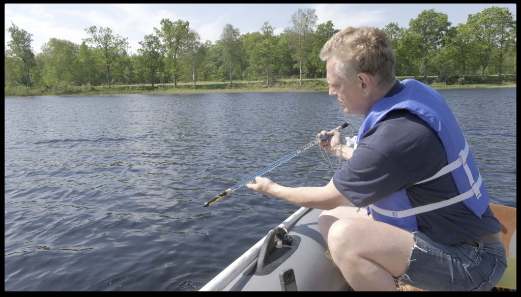
Fast Sediment Profiling Using the SediMeter™ SM4P
In SediSond mode, the SediMeter model SM4P is set up to be a free-fall cone penetrometer. The measurement is triggered by free-fall. It samples for a few seconds at 20 Hz, with the accelerometer running at 400 Hz. As the tip penetrates the sediments the accelerometer records the retardation. At the same time the OBS detectors register the turbidity on their way down. Our software converts these time-series data to a plot of sediment strength and turbidity, with the vertical axis representing elevation (Z). The advantage of this is that the turbidity profile is acquired together with the sediment shear strength data. The low weight of the instrument makes it easy to deploy it from dinghies or canoes, thus enabling field work in the remotest locations.
Field test in a small lake, Sweden
Case 1
This is a rather small lake with dy on just about all bottoms where it is deeper than two feet. The first example was taken in a deep part of the lake with dy and a scattering layer of sediments.
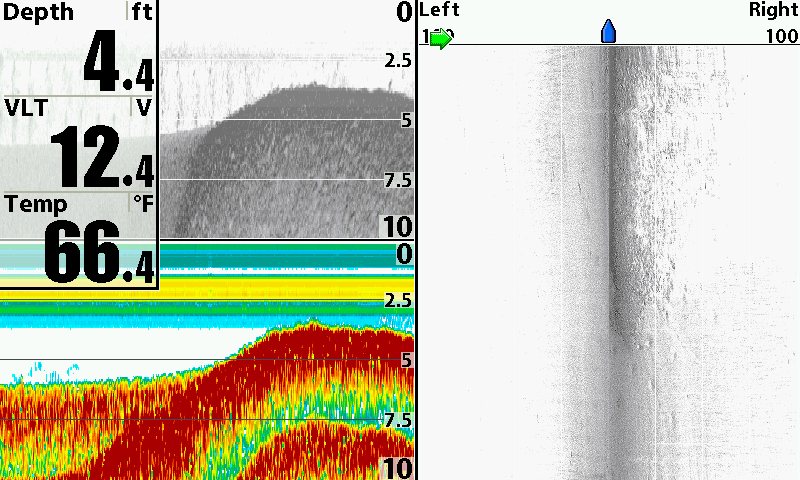
The chart shows 200 and 83 kHz echo-sounders to the left, and 455 kHz side scan sonar to the right.
A sediment profiling was made at this site, and mud came up on the tip.
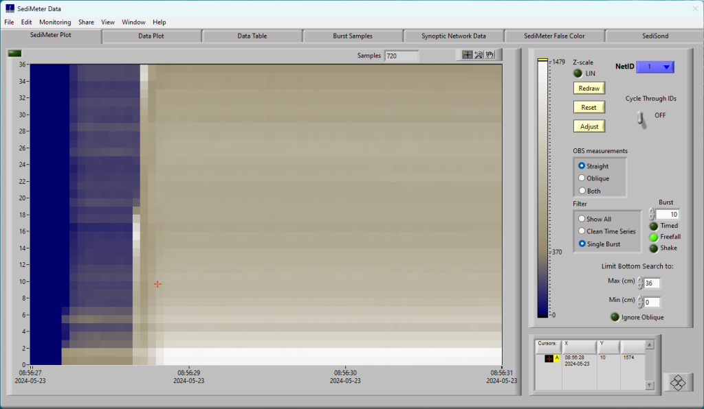
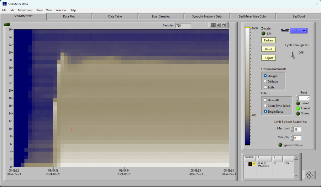
The vertical OBS array intensity chart of the SediSond drop. Note that the sediment surface is lighter (oxygenated) while just a few cm down it because darker (anoxic and gas charged). At the bottom end it is more dense (lighter; what can be seen attached to the tip on the photo).
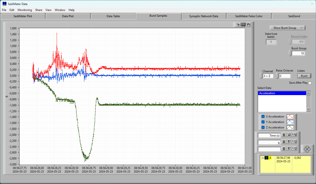
A raw plot of the [X,Y,Z] accelerometer data over time. Note how the Z values go towards 0 during free-fall, and to below -1 g during retardation.
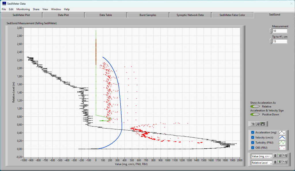
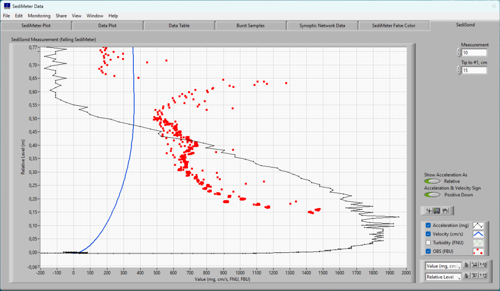
The accelerometer data in black on the x-axis is plotted against the vertical coordinate on the y axis. By integrating the acceleration the velocity is first found (blue line) and then the Z level. The red dots are individual measurements from the 36 OBS detectors, i.e., turbidity.
In this close-up we see how the OBS turbidity data (red dots) compare with the retardation of the probe (black line). In this profiling the entire OBS section got buried inside the sediments, but measurements taken on the way down still leave information about the sediment surface.
Case 2
This site is shallower, the drop was shorter, the velocity lower, and the sediment penetration less.
The site is at the left end, a short distance from a shoal. The sediments are acoustically transparent, and the till bed can be seen through them.
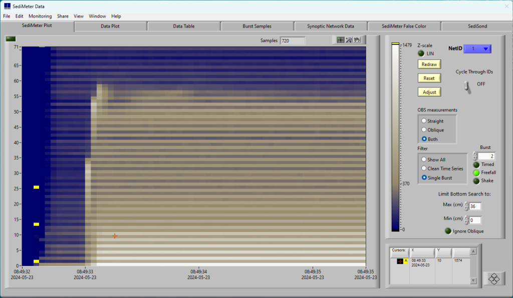
The OBS turbidity profile shows that there were sediments with a higher turbidity as the sensor went down, but the layer is absent after the instrument came to a stop. This is interpreted as the “winter film” that basically behaves like water.
For comparison, this chart shows both the straight backscatter and the oblique reflection data. The difference between the two can be helpful to spot stratification. Also note that a wave was created on the sediment surface. The time window is 3 seconds.
How to Start Using the SediSond™
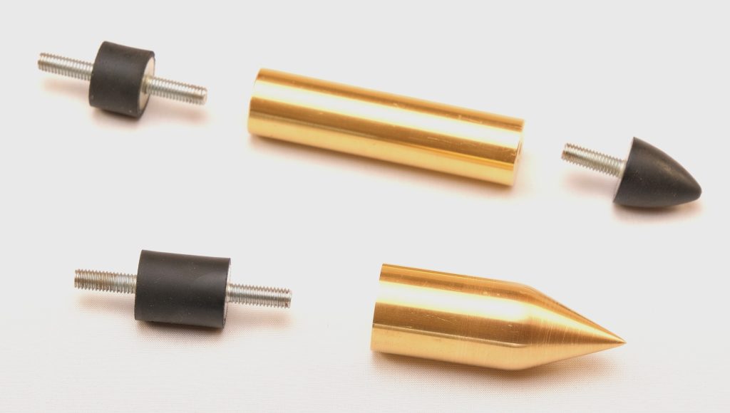
The SediSond™ functionality is present in the SediMeter™ SM4P, and all you need extra is the line attachment and the tip, see photo. The rubber bushings and tip are not just for connection, but also serve as protection against excessive g-forces.
It is also possible to program the SediMeter to act both as a SediSond and as a SediMeter in the same mission. It can be deployed by falling into the bed, recording the free-fall data, and then continue recording as a SediMeter until it is retrieved again.
Near: The standard mounting tip for the SM4P is a 20 mm rubber bushing followed by a 25 mm brass tip. The instrument is pushed down using a tube that acts on this tip. Far: For SediSond™ use we offer this combination of rubber bushing + brass weight + rubber tip. Not shown but also included in the SediSond™ kit is the line attachment.
Cookie Consent
We may use cookies on our site. If we do, this feature is required by law. By using our site, you consent to cookies.
Websites store cookies to enhance functionality and personalise your experience. You can manage your preferences, but blocking some cookies may impact site performance and services.
Essential cookies enable basic functions and are necessary for the proper function of the website.
Name
Description
Duration
Cookie Preferences
This cookie is used to store the user's cookie consent preferences.